
Abstract
Accurate quantification in PET and SPECT requires correction for a number of physical factors, such as photon attenuation, Compton scattering and random coincidences (in PET). Another factor affecting quantification is the limited spatial resolution. While considerable effort has gone into development of routine correction techniques for the former factors, less attention has been paid to the latter. Spatial resolution-related effects, referred to as 'partial volume effects' (PVEs), depend not only on the characteristics of the imaging system but also on the object and activity distribution. Spatial and/or temporal variations in PVE can often be confounding factors. Partial volume correction (PVC) could in theory be achieved by some kind of inverse filtering technique, reversing the effect of the system PSF. However, these methods are limited, and usually lead to noise-amplification or image artefacts. Some form of regularization is therefore needed, and this can be achieved using information from co-registered anatomical images, such as CT or MRI. The purpose of this paper is to enhance understanding of PVEs and to review possible approaches for PVC. We also present a review of clinical applications of PVC within the fields of neurology, cardiology and oncology, including specific examples.
Export citation and abstract BibTeX RIS
General scientific summary Quantification in emission tomography (PET and SPECT) is affected by 'partial volume effects' (PVEs), caused by the relatively poor spatial resolution. PVEs depend on the characteristics of the imaging system and on the object being imaged, and spatial and temporal variations in PVE can often be confounding factors. A number of different methods for partial volume correction (PVC) have been proposed. The best results are obtained by utilising information from anatomical images, such as CT or MRI, which typically have much better spatial resolution provided accurate registration and segmentation of the anatomical modality is achieved. In the past PVC has mainly been used in research studies but as multimodality systems, combining PET or SPECT with CT or MRI, become widely available, PVC can more readily be used in clinical practice. The purpose of this paper is to enhance understanding of PVEs and to review possible approaches for PVC and their application.
1. Introduction and basic concepts
In emission tomography considerable effort has been expended in achieving quantitative reconstruction, accounting for the various sources of bias such as scatter and attenuation as well as instrument-specific parameters such as dead-time, occurrence of random coincidences and non-uniform detection. Spatial resolution in emission tomography, however, is limited and is usually directly coupled to image noise so that any improvements in resolution are accompanied by increased noise. This limited resolution results in quantitative bias when imaging small objects. The purpose of this paper is to enhance understanding of the effects of poor resolution and to review the possible approaches to correct for these effects.
1.1. Partial volume effects
The three-dimensional (3D) distribution of a radioactive tracer inside a patient can be quantified using the functional imaging modalities of positron emission tomography (PET) and single photon emission computed tomography (SPECT). The accuracy of the quantification is limited, however, due to the relatively poor spatial resolution achievable with these modalities. Spatial resolution-related effects are usually referred to as 'partial volume effects' (PVEs). In general the partial volume effect can be defined as the loss in apparent activity that occurs when an object partially occupies the sensitive volume of the imaging instrument (in space or time) (Hutton and Osiecki 1998), a variation on the original definition in Hoffman et al (1979) (see figure 1). Here the sensitive volume refers to the volume defined by the instrument resolution from which emitted photons would be detected at a given detector location (bin).
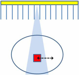
Figure 1. Partial volume effects occur when an object (the small square) partially occupies the sensitive volume (the triangular region) of the imaging instrument (in space or in time). The arrow represents possible motion of the object during acquisition.
Download figure:
Standard imageThe principal PVE in emission tomography corresponds to spill-over of counts (cross-contamination) between different image regions due to the point-spread function (PSF) of the system. This effect is often viewed as two separate effects: spill-in and spill-out, which makes sense when focusing on one target region in which the activity concentration needs to be quantified (e.g. the myocardium in cardiology, brain grey matter tissue in neurology, or a tumour in oncology). Adjacent image regions are then considered as background regions and their activity concentrations are only of interest in relation to their involvement in correctly estimating the target region concentration.
A different type of PVE is the sampling effect related to the voxel size of the images, which in PET and SPECT images is usually several mm per side, depending on application. Each individual voxel can in principle contain two or more tissue types (e.g. blood and myocardial tissue in cardiology, grey matter (GM), white matter (WM) and cerebro-spinal fluid (CSF) in neurology, or tumour tissue and normal tissue in oncology). This can occur at the boundary between regions of different tissue-types, in such a way that a voxel with mixed tissue in principle could be split into a few sub-regions, each with a single tissue type. However, different tissue types could also be mixed on a much finer scale within a voxel, so that such splitting would not be possible (e.g. blood inside small vessels in a tissue region, or air inside the alveoli in lung tissue). This type of PVE is also known as the tissue-fraction effect. When PVE is mentioned in relation to CT or MRI images, it normally refers to the tissue-fraction effect.
Spatial variations in PVE can often be a confounding factor. Pretorius and King (2009) pointed out that PVE can lead to an apparent non-uniformity in perfusion of the myocardium due to a variation in wall-thickness (Pretorius et al 2002). PVE can also be affected by temporal factors. Motion blurring due to cardiac, respiratory or patient motion can cause additional PVEs. Pretorius and King (2008) have shown that respiratory motion compensation is important in relation to PVE correction in cardiac SPECT studies. Correction for motion effects is itself a large area of research and development (van den Hoff and Langner 2012), but is beyond the scope of this review. In dynamic studies (consisting of the acquisition of data in multiple time-frames after the administration of the tracer), the PVE will be affected by changing activity distribution due to uptake and washout of tracer in different tissues or organs. Changes occurring over longer periods of time may also be important. If the size and/or shape of a tumour change over time, PVE will also change, which may be a confounding effect in oncological follow-up studies (Soret et al 2007).
1.2. The point spread function
The spatial resolution is usually characterized by the point-spread function (PSF), which essentially corresponds to the image of a point source. In general the PSF in SPECT and PET images is spatially variant—meaning that the distribution of values around the position of the point source depends on the location of the source in the field of view (FOV) of the scanner. In many situations, however, it is reasonable to assume that the PSF is position-invariant. This is all the more true when images are reconstructed by taking into account the variation of the detector response as a function of position of the source with respect to the detector, as now implemented both in SPECT (e.g. Zeng et al 1991, Vija et al 2003) and PET (e.g. Panin et al 2006, Sureau et al 2008, Alessio et al 2010). In this case, the reconstructed PET or SPECT image can be described as a convolution of the true activity distribution with the PSF. The PSF itself can often be modelled as a Gaussian function, uniquely defined by its full width at half maximum (FWHM), which can be different in different spatial directions. Alternative models describing the PSF in the reconstructed images have also been described though (e.g. Taschereau et al 2011).
The Fourier transform of the PSF is known as the modulation transfer function (MTF). The MTF contains the same information as the PSF, but expressed in the frequency domain rather than in the spatial domain. The Fourier transform of a Gaussian function is also a Gaussian function, and the widths of the two functions have an inverse correlation: as the spatial domain Gaussian becomes broader, the frequency domain Gaussian becomes narrower, and vice-versa (see figure 2). The operation of convolution with a PSF in the spatial domain is equivalent to multiplication with the corresponding MTF in the frequency domain. This means that a PET or SPECT image can be described in the frequency domain as the product of the Fourier transform of the true activity distribution and the MTF of the system. Image components corresponding to mid-range frequencies, although attenuated, may still be present in the data and could in principle be restored by an inverse filtering operation. On the other hand, image components at higher frequencies, where the MTF is essentially zero, will be lost forever from the data. Attempts to restore these image components usually lead to noise-amplification or image artefacts.
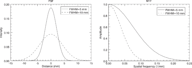
Figure 2. Point spread functions with FWHM of 5 and 10 mm (left), and corresponding modulation transfer functions (right).
Download figure:
Standard image1.3. Partial volume correction
The ultimate goal of partial volume correction (PVC) is to reverse the effect of the system PSF in a PET or SPECT image and thereby restore the true activity distribution, qualitatively and quantitatively. This can be done by deconvolution, either in the image domain or during iterative image reconstruction by incorporating the PSF in the system matrix. The first approach results in noise amplification, while the second approach has a superior noise performance. This is because a larger number of measured data values are involved in the reconstruction of each voxel value, resulting in noise averaging. In both cases, however, the resulting images often suffer from so called 'Gibbs artefacts', corresponding to ringing in the vicinity of sharp boundaries, which is related to missing high frequency information. This could be caused by information loss during data acquisition due to limitations in the detector system design, or by insufficient sampling in the image domain by the use of too large voxels. The main advantage of these methods is that they depend on PET or SPECT data only, and no other data set is needed. This is, however, also a limitation.
As pointed out by Strul and Bendriem (1999), because of the ill-conditioned nature of the restoration problem, some sort of regularization must be used to avoid high-frequency noise-amplification and introduction of artefacts, and this can be achieved by incorporating anatomical information and tissue homogeneity constraints. The aim of anatomically based PVC methods is to utilize structural information from other imaging modalities as a priori information in order to stabilize the solution. This leads to a synergistic combination of the two data sets, with resultant benefit.
The first step in anatomically based PVC is to segment and/or parcellate the anatomical image into a number of compartments or regions that are usually considered to be functionally 'uniform'. This does not mean that the activity concentration has to be identical at each point in a region—only that the variability within a region should be small in comparison to the potential variability between different regions. The uniformity assumption is an approximation used for the purpose of calculating the PV correction factors. The assumption implies that there is a PVE-equilibrium within each region; i.e. the net-effect of the cross-talk between voxels within one single region is negligible. In practice, this means that the correction is performed between voxels in different regions, but not between voxels in the same region. PVC should thus be considered, not as an exact correction method, but as a first order approximation.
In section 2 various PVC methods developed over the years will be described. In section 3 the application of PVC in neurology, cardiology and oncology will be discussed and some clinical examples provided. Some of the acronyms used in this paper are explained in table 1. Although this paper is primarily concerned with describing the algorithms and the accuracy of various approaches to PVC, it should be kept in mind that the precision of quantitative estimates can often be equally important as accuracy.
Table 1. Most commonly used acronyms.
| Acronym | Meaning |
|---|---|
| AD | Alzheimer's disease |
| CBF | Cerebral blood-flow |
| CSF | Cerebro-spinal fluid |
| FDG | Fluoro-deoxy glycose |
| GM | Grey matter |
| GTM | Geometric transfer matrix |
| LV | Left ventricle (of heart) |
| MGM | Müller-Gärtner method |
| PSF | Point spread function |
| PVC | Partial volume correction |
| PVE | Partial volume effect |
| RBV | Region-based voxel-wise correction |
| RC | Recovery coefficient |
| ROI | Region of interest |
| RV | Right ventricle (of heart) |
| SUV | Standard uptake value |
| VOI | Volume of interest |
| WM | White matter |
2. PVC techniques
PVEs depend on a number of different factors, such as the target organ size, the type of scanner used, the spatial resolution, the activity distribution, as well as motion and other temporal effects. Therefore a range of different correction techniques have been developed over the years, and there is probably not one single technique that would be optimal in all imaging scenarios. A comparison of different approaches was also presented by Hutton et al (2006a) and by Soret et al (2007). In the description below we have tried to include most of the PVC methods developed in the past. These are presented under the following subsections: image enhancement techniques, which primarily rely on recovering resolution directly from the emission data (section 2.1), image-domain correction techniques that rely on anatomical information (or experimental findings) to determine appropriate correction (section 2.2) and projection-based correction (section 2.3). We also specifically address PVC for non-uniform regions (section 2.4), corrections for tissue fraction (section 2.5) and application to dynamic data (section 2.6). Finally a comparison of a few different PVC methods, based on simulated data, is given (section 2.7).
In the following we will use the terms region, region of interest (ROI) or volume of interest (VOI) interchangeably referring to a 3D sub-region in the image domain. The terms mask and template will also be used referring either to a single region or to a set of regions, depending on the context.
2.1. Image enhancement techniques
Reversing the effect of the imaging system point spread function can be performed using two main approaches: image reconstruction with resolution modelling and/or introduction of anatomical priors, and post-reconstruction image restoration.
2.1.1. Enhancing spatial resolution during reconstruction
An effective method to enhance the spatial resolution in reconstructed SPECT and PET images is to incorporate the PSF into the system matrix used for forward and back-projection (see e.g. Tsui et al 1994, Liow et al 1997, Hutton and Lau 1998, Pretorius et al 1998, Zeng et al 1998, Reader et al 2003). Inclusion of resolution in the system matrix (model) is now available as an option on most SPECT and PET systems and therefore immediately applicable. It should be noted, however, that the application of this more exact model of the system is mainly used in practice to reduce the noise in the reconstruction, improved noise properties being a by-product of the improved system model. Although in theory the inclusion of the resolution aims to reconstruct the exact activity distribution, there is a limit to the recovery achievable, even at high iterations, due to the loss of high frequency information during data acquisition. Recovery is therefore limited since there will still be residual partial volume effects, that can be hard to estimate, given the nonlinear nature of the reconstruction. At best, partial volume effects are reduced in magnitude provided a sufficient number of iterations are performed, but quantitative recovery is limited.
Better results can be obtained with reconstruction algorithms involving anatomical priors to control noise and enhance edges between functional structures (most often assuming that edges between two functional compartments match the edges between two anatomical compartments). Visually these techniques can produce very striking image contrast. There is, however, rather limited reference to the effectiveness of these techniques in achieving quantitative PVC.
When using penalized iterative reconstruction algorithms (including Bayesian or maximum a posteriori (MAP) algorithms), a smoothness prior is often used. This encourages solutions with a low degree of variability between adjacent image voxels. With a segmented anatomical image, the smoothness constraint can be restricted to each anatomical region, and larger differences can thereby be allowed between adjacent voxels belonging to different regions. This is the basic principle used by most groups in the past. Early work includes Chen et al (1991), Fessler et al (1992), Gindi et al (1993) and Ouyang et al (1994).
Ardekani et al (1996) developed a method based on minimisation of cross-entropy, which utilized multi-spectral MRI data. Bowsher et al (1996) presented a Bayesian method for simultaneous reconstruction and segmentation of PET or SPECT data, in which higher prior probabilities were assigned when segmented regions stayed within anatomical boundaries. Lipinski et al (1997) presented a method that assumes a Gaussian distribution of the image values with the same mean value for all voxels within a given anatomical region. Sastry and Carson (1997) presented a MAP algorithm based on a tissue composition model, in which the image is described as a sum of activities for different tissue types, determined from a segmented MR image. Comtat et al (2002) presented an algorithm for reconstructing whole-body PET/CT data, in which the anatomical labels were blurred in order to take into account the uncertainty associated with the anatomical information. This method was later also applied to brain studies by Bataille et al (2007). Baete et al (2004) presented a MAP reconstruction algorithm for brain PET studies using a tissue composition model, in which WM and CSF were treated as uniform for the purpose of estimating the GM values. Bowsher et al (2004) described an algorithm based on an image model promoting greater smoothing among nearby voxels that have similar MRI signals, which therefore did not require segmentation of the anatomical image. Alternative methods, based on an anatomically driven anisotropic diffusion filter, were presented recently (Yan and Yu 2007, Chan et al 2009, Kazantsev et al 2012). Another novel approach was presented by Pedemonte et al (2010), in which a hidden variable is introduced, denoting tissue composition that conditions a similarity function based on entropy.
More work needs to be undertaken in order to better understand the sensitivity of these methods to mis-matched anatomical information (whether due to mis-registration or simply lack of functional/anatomical correspondence). Application has been largely in neurological studies where registration tends to be straightforward.
2.1.2. Post reconstruction image restoration
The second approach consists of performing an image enhancement by post-processing the image reconstructed without resolution modelling (or in an attempt to reduce residual partial volume effects after reconstruction with resolution modelling). This can be performed either using a deconvolution operation on a reconstructed image, or by incorporating into the reconstructed image some high frequency information taken from a structural image.
In the deconvolution approach, the blurred image is described as follows:

where b( · ) is the uncorrected image, a( · ) is the true image, h( ·, ·) is the PSF, which can be space variant or invariant, and x and y are 3D coordinates. (When no integration limits are specified, it means that the integration is to be performed over the whole space.)
Various iterative techniques have been used for image restoration: Teo et al (2007) and Tohka and Reilhac (2008) used the Van Cittert deconvolution technique, Tohka and Reilhac (2008) also used the Richardson–Lucy algorithm, and Kirov et al (2008) and Barbee et al (2010) used the MLEM algorithm. As an example, the reblurred Van Cittert iterative scheme, can be described as follows (Tohka and Reilhac 2008):

where  is the corrected activity distribution after k iterations, α is the step-length, in practice usually selected close to 1, and ⊗ represents the convolution operator. Here h( ⋅ ) is assumed to be a position-invariant PSF. The goal of this algorithm is to find the activity distribution (ãk) such that the blurred distribution (h ⊗ ãk) matches the observed distribution (b) in a least squares sense. The formula arises since minimizing (b − h ⊗ ãk)2 is achieved when its derivative
  is zero. The basic idea of the iterative scheme is to detect structures in the residual (b − h ⊗ ãk), and to put these back into the restored image. The process starts with the observed image and finishes when no more structures are detected.
Hoetjes et al (2010) compared post-reconstruction deconvolution with reconstruction-based resolution recovery for oncological PET studies, and found the two approaches had similar accuracy, but the reconstruction-based method had better precision.
The main problem with the deconvolution-based methods is the need to control noise by regularizing the solution (e.g. post-reconstruction smoothing (Boussion et al 2009)). Consequently with realistic noise levels it is very difficult to achieve full resolution recovery (indeed impossible given the high frequency losses that occur during acquisition). As a result full partial volume correction cannot be achieved. In order to address this problem, Bousse et al (2012) recently presented a maximum penalised likelihood deconvolution technique, based on a model that assumes the existence of activity classes that behave like a hidden Markov random field driven by a segmented MRI image.
An alternative to performing deconvolution is an approach that consists of transferring high-frequency information directly from a high-resolution anatomical image to a PET or SPECT image. Calvini et al (2006) proposed a method in which high-frequency information was extracted by subtracting a blurred version of an MRI image from the original one. These data were weighted and then added to a SPECT image. Boussion et al (2006) propose a more sophisticated method, in which the high frequency information was transferred in the wavelet domain from a CT or MR image to a PET or SPECT image. One advantage with this approach is that it does not require segmentation of the anatomical image. A potential disadvantage is that artefacts may be introduced in areas where there is mismatch between the structural and functional images, although this problem can be reduced using a local analysis approach (Le Pogam et al 2011). Shidahara et al (2009) showed that improved performance could be obtained by using a segmented anatomical image instead of the raw CT or MR image. However, if segmentation is required after all, it may be preferable to choose a method based on a more solid theoretical foundation.
2.2. Image domain anatomically based PVC techniques
PVC techniques that utilize anatomical information can be divided into several groups; in some techniques only the mean value in a region is estimated, while in other techniques the correction is performed for each individual voxel; also in some techniques the correction is only done for one single region (the target region), while in other techniques the entire image is corrected.
2.2.1. Mean value correction—single region
In one of the first works on PVC for PET, Hoffman et al (1979) defined the recovery coefficient (RC) as the apparent activity concentration of an object divided by its true concentration. The RC could be calculated based on the system PSF and the geometry of the object. The authors determined the RC for objects of different sizes and shapes scanned on their PET system, and found it to be strongly dependent on object size. The RC concept was introduced in Hoffman et al (1979), but no mathematical expression was provided. Below we derive such an expression. In all equations below, variables with a tilde (e.g.  ) represent an estimation of the corresponding variable without tilde (e.g. A).
The mean value of an image b inside a region Ω is defined as follows:

Using (1) we get:

Assuming a( · ) to be approximately constant inside Ω, with a mean value of AΩ, and zero outside leads to:

The true regional mean value can then be estimated as:

where R is the RC value, defined as:

The RC values from Hoffman et al (1979) were used by Wisenberg et al (1981) to quantify myocardial blood flow in dogs with PET. The wall-thickness, needed for selecting the appropriate RC values, was determined from echocardiographic measurements. Kessler et al (1984) determined RC values for objects of various shapes and various dimensions with non-zero background. The RC definition can be based either on the mean apparent activity concentration in the target, or on the maximum activity concentration in the target, e.g. Srinivas et al (2009).
In oncological applications, it is a common practice to experimentally determine recovery coefficients using spherical phantom inserts. In this case, the correction would only be theoretically applicable to spherical lesions. However, the determination of recovery coefficients as described above is valid for any shape of the volume concerned (provided known).
Although the RC-based correction was initially proposed assuming that the target could be delineated using a structural imaging modality (CT or MR), it can be extended to be applicable without such structural information (Avril et al 1997, Gallivanone et al 2011). In that case, the volume of the target is directly estimated from the PET image, using a threshold-based method.
2.2.2. Mean value correction—multiple regions
The method initially described in Hoffman et al (1979) corrects only for the spill-out effect. To correct for both spill-out and spill-in, the approach described above can be extended to multiple regions. Assuming a( · ) to be approximately piece-wise constant, with mean value Ai in region Ωi, equation (5) becomes:
where M is the number of regions and ϕij are the cross-talk factors, defined as:

(Note that Ri = ϕii). With a matrix formulation, the solution to this system of equations is given by:

where  and B are the vectors of estimated and uncorrected regional mean values, respectively, and ϕ = [ϕij] is a matrix containing the cross-talk factors. This method was first introduced by Henze et al (1983). They developed the technique to correct for cross-contamination between the myocardium and the left ventricular blood-pool. Although these authors used only two regions (M = 2), the technique they described would be valid for any number of regions. The method from Henze et al (1983) was applied by Herrero et al (1988) in myocardial blood flow PET studies on dogs. This method later became known as the 'geometric transfer matrix' (GTM) method, after it was described by Rousset et al (1998) for application to the brain.
The GTM method is widely applied for regional analysis and has the advantage that it can account for spillover effects between multiple regions. The main disadvantage is that the method only provides mean values for the predetermined regions but does not provide a partial volume corrected image.
2.2.3. Voxel-based correction—single region
A voxel-based PVC method was developed by Videen et al (1988), using anatomical information from either CT or MRI. The method was developed for brain PET studies, and the anatomical image was segmented into two regions; a brain region (including both GM and WM) and a non-brain region (including CSF). The latter was assumed not to contain any tracer. A binary map of the brain region was convolved with the system PSF to generate an image of RC values for each voxel. PVC was then performed by dividing the original PET image with the RC map, considering only voxels within the brain region. From (1) we obtain, with the assumption that  and zero elsewhere:

The correction can then be described as follows:

where r( ⋅ ) is the distribution of recovery factors for each voxel:

Please note that AΩ does not appear in the final correction formula. This method is essentially an extension of the RC-method (6) (Hoffman et al 1979) from a regional to a voxel basis. In Videen et al (1988) the method was illustrated with 2D simulations, but the authors stated that, with real data, the correction must be applied in 3D. This was later done by Meltzer et al (1990).
Müller-Gärtner et al (1992) extended the voxel-based Videen method (described above) from two to three regions in order to account for WM and to get more accurate GM values. An MRI image of the brain was segmented into GM, WM and CSF regions. The GM region was treated as the target region, and the other two as background regions. CSF was assumed to be devoid of activity. The binary WM map, scaled to an estimate of the true WM mean value, was convolved with the system PSF and subtracted from the original PET image. Finally, corrected values were obtained for GM voxels as described above for the Videen method. We will refer to this method as MGM (short for 'the Müller-Gärtner method'). If indices 1 and 2 represent GM and WM, respectively, we obtain from (1):

If  where
where  is an estimate of the mean value in the background region (WM), the correction can be described as follows:

where r1( · ) is the distribution of RC values in Ω1:

and ϕ2( · ) is the distribution of cross-talk factors from Ω2 in Ω1:

This scheme can easily be extended to include multiple background regions:
where M is the total number of regions. This method has similarities to scatter and attenuation correction used in PET and SPECT: first there is a subtraction of events that are misplaced into the target region (similar to scatter correction), and then a multiplicative correction is applied for events that are lost from the target region (similar to attenuation correction). The disadvantages with this method are that; (1) the correction is valid only for voxels within the target region, and (2) the true mean values in the background regions  have to be initially estimated. These would typically be obtained from regions large enough that the central part can be assumed to be unaffected by PVE. An alternative would be to use the GTM method to determine the mean values of the background regions, as described in Quarantelli et al (2004). This is known as the modified MGM (mMGM). Figure 3 illustrates MGM applied to a 1D phantom profile.
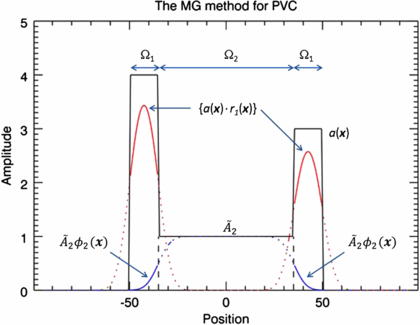
Figure 3. Illustration of the MG method (15) (Müller-Gartner et al 1992). The correction is applied only in the target region, Ω1. Spill-in correction is done by subtracting a background term  . Spill-out correction is achieved by dividing by r1(x). The true mean value,
  , in the background region, Ω2, has to be initially estimated. The black solid line represents the true distribution. The red and blue lines represent the result of convolving the target and background regions separately by the PSF. The solid portion of these curves represents the data used in the algorithm.
Download figure:
Standard imageMGM is one of the most used PVC methods. Originally developed for brain PET studies, it was implemented for brain SPECT studies by Matsuda et al (2003). It was also implemented for cardiac SPECT studies by Da Silva et al (1999). These authors developed a new method for deriving the cross-talk and recovery factors in order to take into account the distance-dependent resolution of the SPECT camera. Instead of convolving regional maps by a Gaussian PSF, the regional maps were forward projected with a model that included attenuation and distance-dependent resolution, and then reconstructed. In Da Silva et al (1999) the method was evaluated with phantom data, and later it was also applied to real data from animal studies (Da Silva et al 2001).
There are thus two methods to calculate the cross-talk and recovery factors: either by convolving the binary maps of the region of interest by the PSF of the imaging system, or by forward projecting and then reconstructing the binary map of the regions using a realistic forward model and the same reconstruction method as the one used for the data to be later corrected. These two methods were compared for brain PET studies by Frouin et al (2002) and for brain SPECT studies by Soret et al (2003). In both cases, no significant difference was found between the two methods. The method based on forward-projection and reconstruction of regional maps is in principle only valid when analytical reconstruction algorithms (e.g. filtered backprojection (FBP)) are used. Iterative algorithms are nonlinear and the result depends on the activity distribution. This means that the reconstruction of a regional map in isolation will produce a different result than if it had been part of a larger object. A solution to this problem was proposed by Du et al (2005) and by Boening et al (2006) using a perturbation technique. Two images with a small difference are forward-projected and reconstructed, and the difference of the two reconstructed images corresponds to the map of correction factors. Pretorius and King (2009) pointed out a limitation with this approach. They observed that when local differences in uptake exist between the emission data and the added forward projected regional map, such as in the case of a cardiac perfusion defect, the map of the correction factors (difference of the two reconstructed images) erroneously takes on some of the characteristics of the emission data.
2.2.4. Voxel-based correction—multiple regions
One of the disadvantages of MGM is (as mentioned before) that the correction is valid only for voxels within the target region. Yang et al presented a method where PVC is applied to the whole image (Yang et al 1996). In this method, a piece-wise constant image is created, where each region is represented by its true relative mean value (Ari = Ai/A1∀i), where A1 is the mean value in an arbitrary reference region. This image is convolved with the system PSF, and PVC factors were obtained as the ratio of the two images (before and after convolution). The convolved piece-wise constant image can be described as:

and the correction is then given by:

where

or

and ac( ⋅ ) is a piece-wise constant image (the subscript c indicating a constant distribution within each region):

This method is essentially an extension of the Videen method (12) from one to multiple regions. The method requires knowledge of the true relative activity concentrations in all regions, which is a strong prior. Absolute values are not needed, as any scaling factor would just come out in the wash. In Yang et al (1996), the method was applied to brain blood flow studies to correct for cross-talk between the GM, WM and CSF regions, which were assigned relative mean values of 4, 1 and 0, respectively. Figure 4 illustrates the Yang method on a 1D phantom profile.

Figure 4. Illustration of the Yang method (20) (Yang et al 1996). Spill-in and spill-out effects are corrected for simultaneously as a multiplicative correction. The true relative mean values,  , in all regions have to be known in advance. The black solid line represents the true distribution. The blue solid line represents the distribution with the
  values in each region convolved with PSF. The dotted line represents the correction factors c(x). The dashed line represents unity.
Download figure:
Standard imageShcherbinin and Celler (2010) implemented this method for SPECT using forward projection and reconstruction to generate  in the calculation of the PVC factors instead of convolving with a PSF. The correction was applied to phantom data using the known activity concentrations in the different compartments for Ari.
Both MGM and the Yang method suffer from the drawback of requiring initial information in terms of mean or relative mean values in various regions. Novel approaches have been proposed which avoid this problem by combining MGM and the Yang method, respectively, with the GTM method.
An extension of MGM was proposed by Erlandsson et al (2006). The first step of this 'multi-target correction' (MTC) method is to use the GTM method to obtain estimates of the true mean values in all regions  . Next, the MGM formula with multiple background regions (18) is applied repeatedly, so that each region in turn is treated as the target region while all other regions are considered as background regions. Thereby, all regions would be considered alternatively as a target or background regions. The final image is obtained as a mosaic of all the corrected regions. The correction of each region is independent of that of all other regions.
Thomas et al (2011a) presented a modified version of the Yang method called 'region-based voxel-wise correction' (RBV). The regional mean values  are initially obtained using GTM, and the Yang correction (20) is then applied. The results obtained are similar to MTC, but RBV is simpler to implement. Instead of using GTM, the mean values in all regions can be estimated with an iterative procedure as follows. The correction is first applied with
  , then new regional mean values are calculated and a new correction applied, etc. As only a few iterations are needed (typically 3–5), this procedure is faster than RBV and simpler as well. This approach is presented here for the first time. We call it the 'iterative Yang' (iY) method. These methods produce a voxel-by-voxel correction of the whole image, do not require any prior information about the activity distribution and can be used with any number of regions. A comparison of the MGM, GTM and RBV methods is presented in the example below (section 2.7).
Shcherbinin and Celler (2011a) also presented a new algorithm, based on the Yang method (Yang et al 1996), which can be described as follows: a template image is calculated based on an initial image reconstructed without PVC and on a structural image. The voxel values in the target region of the template are set to a constant equal to the mean of the top ten percentile voxels in the corresponding region of the original image while the background values are set to their values in the original image. The template is projected and reconstructed to mimic the detection/reconstruction process. The voxel values in the target region are then corrected by multiplying them by correction factors, as in (20). These factors are equal to the ratio of the template values to the values in the images reconstructed from the template projections, similar to (21). The corrected target region is then projected again and the result is used to update the background estimate. Two iterations are performed to get the PVC image. This method has been called the 'iterative partial volume effect correction' (itPVEC) method.
2.3. Projection based PVC
None of the PVC methods presented above explicitly uses known properties of the image noise distribution but, according to Aston et al (2002), different PVC methods have different implicit assumptions about the underlying noise model, and these assumptions may affect the precision of the correction. Various authors have described expressions for estimating the co-variance in reconstructed tomographic images (Barrett et al 1994, Qi 2003). However, this is not trivial, especially for iterative reconstruction methods. On the other hand, in the projection domain the noise distribution is known to follow the Poisson model, and this knowledge can be utilized by methods operating in the projection domain.
2.3.1. ROI reconstruction methods
Huesman (1984) developed an analytic algorithm to obtain ROI mean values directly from projection data, without reconstructing the complete image. Carson (1986) developed an iterative ML-EM algorithm for the same purpose. By incorporating the resolution of the scanner into the algorithm, PV corrected ROI mean values were automatically obtained. An alternative approach, based on least-squares algorithm was developed by Formiconi (1993). This algorithm was evaluated with brain SPECT studies on phantoms and patients by Vanzi et al (2007). These methods require segmentation of the entire object. In order to avoid this, Moore et al (2012) developed a method, which only requires segmentation of few tissue types (2 to 4) within a small sub-VOI surrounding the lesion seen on the CT or MR structural image. Only the projection rays traversing the VOI are used to estimate the mean activity concentration in each tissue type. These activity concentrations are estimated simultaneously by maximizing iteratively the log likelihood of measuring a given projection dataset. The contribution of the background outside the VOI is accounted for by reprojecting through the reconstructed image outside the VOI. One advantage of this method is that, being based on maximum-likelihood fitting in projection space, it utilizes the knowledge that the projection noise is white (spatially uncorrelated) and Poisson distributed.
2.3.2. Voxel-based PVC from projections
In all the anatomically based PVC methods discussed above, the correction is performed in the image domain. The correction can actually also be performed in the projection domain, as described in Erlandsson and Hutton (2010) and Erlandsson et al (2010, 2011) for SPECT, still requiring the segmentation of the different tissue types from a structural CT or MR image. The original method by Erlandsson and Hutton (2010) was developed in combination with iterative FBP reconstruction. A second version that worked in combination with OSEM reconstruction (Hudson and Larkin 1994) was later presented by Erlandsson et al (2010, 2011). In these approaches, the projection domain is related to the image domain by the forward-projection operator:


where p(θ) and pR(θ) are projection data sets without and with resolution blurring, respectively, F{ ⋅ } and FR{ ⋅ } represent the forward-projection operator without and with resolution modelling, respectively, and θ is a coordinate in the projection domain. The projection space correction is based on the Yang approach (Yang et al 1996), and can be described as follows:

where ac( ⋅ ) is a piece-wise constant image:

New mean value estimates  are calculated after each iteration of the reconstruction algorithm. The main advantage of this method is that it takes into account the distance dependent resolution in SPECT.
2.4. Non-uniform PVC
A limitation of the anatomically based PVC approaches has been the assumption that the selected regions, defined anatomically, have uniform activity. In Erlandsson et al (2010) it was shown that, although violation of the uniformity-assumption resulted in bias, some information about the underlying distribution was maintained in the image. Shcherbinin and Celler (2011b) showed that even if PVC methods based on the uniformity assumption perform at best when the true activity is uniformly distributed throughout the target region, they still improve the total activity estimates when the true activity distribution is non-uniform.
Some of the methods presented above allow for the possibility for going beyond the simple uniformity assumption. Erlandsson and Hutton (2011) presented a voxel-based PVC method, based on hyper-planes, which allows for a gradient in the activity distribution within each region. The method is based on the iterative Yang algorithm, described above. At each iteration a hyper-plane (described by the mean value,  , and a 3D gradient vector,
  ) is fit to the data within each region. The hyper-planes are then used instead of uniform distributions for calculation of the correction factors, c(x), using (21b) with ac( ⋅ ) replaced by ag( ⋅ ):

where xci is the centre of region i. This technique could also be extended to more complex analytical functions for describing the basic distribution, but then the number of parameters to estimate would increase.
The method by Moore et al (2012), described above, was initially designed assuming the activity concentration was uniform in each tissue type. However, it has recently been extended to incorporate a model of non-uniform activity distribution in the target tumour region (Southekal et al 2011). The model assumes a radially varying non-uniform uptake, and was supposed to describe tumours with a necrotic core. Two parameters instead of one are thus estimated for the target region.
Another approach for dealing with the case of non-uniform distribution within anatomically defined regions is the 'segmentation modifying PVC' (SM-PVC) method, developed by Thomas et al (2011b). This method automatically alters the defined sub-regions based on the emission data so as to best match the assumption of constant activity within regions, in preference to relying on anatomical partitioning. This potentially could be extended to permit in some applications atlas-based segmentation without the need for a patient-specific anatomical image set.
Some of the properties of various PVC methods are summarised in table 2.
Table 2. Summary of properties of different PVC methods, including whether PVC is applied on regional mean-values or on the voxel-values, whether PVC is applied to a region or to the whole image, whether correction is done for both spill-in and spill-out or only for spill-out, whether the uniformity assumption is used or not, whether an anatomical prior is used or not, whether the algorithm operates in the image or in the projection domain, as well as whether prior information about the activity distribution is required or not.
| PVC method | Region-/voxel-based | Region/image Corr. | Spill-in/spill-out corr. | Uniform assump. | Anat. prior | Image/projection domain | Prior info. req. |
|---|---|---|---|---|---|---|---|
| RR-recon | Vox | Im | S-I + S-O | No | No | Pr | No |
| AP-recon | Vox | Im | S-I + S-O | Yes/No | Yes | Pr | No |
| Post-deconv | Vox | Im | S-I + S-O | No | No | Im | No |
| AP-post-dec | Vox | Im | S-I + S-O | No | Yes | Im | No |
| Wavelet | Vox | Im | S-I + S-O | No/Yes | Yes | Im | No |
| RC | Reg | Reg | S-O | Yes | Yes | Im | No |
| GTM | Reg | Im | S-I + S-O | Yes | Yes | Im | No |
| V-RC | Vox | Reg | S-O | Yes | Yes | Im | No |
| MGM | Vox | Reg | S-I + S-O | Yes | Yes | Im | Yes |
| fp-MGM | Vox | Reg | S-I + S-O | Yes | Yes | Pr/Im | Yes |
| p-GTM | Reg | Im | S-I + S-O | Yes | Yes | Pr/Im | No |
| Y | Vox | Im | S-I + S-O | Yes | Yes | Im | Yes |
| MTC,RBV, iY | Vox | Im | S-I + S-O | Yes | Yes | Im | No |
| itPVEC | Vox | Reg | S-I + S-O | Yes/No | Yes | Pr/Im | No |
| ROI-recon | Reg | Im | S-I + S-O | Yes | Yes | Pr | No |
| VOI-fit | Reg | Reg | S-I + S-O | Yes | Yes | Pr | No |
| p-PVC | Vox | Im | S-I + S-O | Yes | Yes | Pr | No |
| OSEM-PVC | Vox | Im | S-I + S-O | Yes | Yes | Pr | No |
| NU-PVC | Vox | Im | S-I + S-O | No | Yes | Im | No |
| SM-PVC | Vox | Im | S-I + S-O | Yes | Yes | Im | No |
Correction methods: RR-recon = reconstruction with resolution recovery, AP-recon = reconstruction with anatomical prior, Post-deconv = post-reconstruction deconvolution, AP-post-dec = post-deconv with anatomical prior, Wavelet = wavelet-domain enhancement, RC = recovery coefficient, GTM = geometric transfer matrix, V-RC = voxel-based RC, MGM = Müller-Gärtner method, fp-MG = forward-projection and reconstruction MGM, p-GTM = perturbation GTM, Y = Yang method, MTC = multi-target correction, RBV = region-based voxel-wise correction, iY = iterative Yang, itPVEC = iterative PVE correction, ROI-recon = ROI reconstruction, VOI-fit = VOI-fitting approach, p-PVC = projection-based PVC, OSEM-PVC = p-PVC with OSEM reconstruction, NU-PVC = non-uniform PVC, SM-PVC = segmentation-modifying PVC.
2.5. Tissue fraction correction
Much less work has been undertaken to address the tissue fraction problem. A method to determine tissue fraction in lungs was presented by Rhodes et al (1981). The extra-vascular lung tissue density was determined by subtracting a blood-volume image from a transmission scan. Spinks et al (1991) presented a PVC method for cardiac PET studies based on extra-vascular tissue density estimated as described in Rhodes et al (1981) and this method was later implemented for cardiac SPECT by Hutton and Osiecki (1998). Iida et al (1991) compared the concepts of extra-vascular tissue density (Rhodes et al 1981) and tissue fraction (Iida et al 1988) (see below), and found they were similar but not identical. Tissue fraction includes a venous component, while extra-vascular density includes non-perfusable (necrotic) tissue.
A method to correct for tissue-density variations in PET/CT studies of lung was recently implemented by Lambrou et al (2011), reducing the intra-subject and inter-subject variability in standardized uptake values (SUV). The effect of differences in air volume for normal and diseased lung is potentially eliminated by means of this technique although further correction would be necessary for other possible tissue compartments (e.g. blood vessels, fibrotic tissue).
Boening et al (2006) describe an extension of the method from Da Silva et al (1999), in which edge voxels were treated as a mixture of the two tissue types. This method was later evaluated in simulated cardiac perfusion SPECT studies by Pretorius and King (2009) where edge voxels were treated as a mixture of two or more tissue types (liver, lung, myocardium, or blood pool) depending on location.
2.6. PVC of dynamic data
In kinetic analysis of dynamic PET or SPECT studies, the contribution from activity in the blood is usually subtracted from the measured tissue time-activity curves, based on data from blood samples taken during the experiment. The fractional blood volume is either assumed to be a predetermined constant (e.g. 5% in brain studies (Mintun et al 1984)) or is treated as an extra parameter to be determined as part of the analysis (see e.g. Erlandsson 2011, Bentourkia 2011).
Iida et al (1988) developed a voxel-based PVC method specifically for dynamic myocardial blood flow PET studies with H215O, which could correct for the tissue fraction effect as well as for the wall-motion of the myocardium. First, the contribution from circulating blood was removed by subtracting a blood-volume image (obtained from a C15O scan) scaled to the arterial concentration at each time frame (obtained from arterial sampling). The tissue fraction (α) was corrected for in the kinetic modelling process, by assuming that the blood-to-tissue partition coefficient (p) for the tracer (H215O) was known: α = (K1/k2)/p. Later, the method was also applied to brain PET studies with separate modelling of GM and WM by Iida et al (2000).
PVC is also important for estimation of image derived input functions, especially when small blood vessels must be used, such as the carotid arteries in the case of brain studies (Zanotti-Fregonara et al 2009). Fang and Muzic (2008) presented an interesting approach for analysing dynamic data from small animal cardiac studies, in which PVC and kinetic modelling were performed simultaneously. VOIs were generated for the left ventricular cavity and myocardium. The cross-talk and recovery factors for the two ROIs were then estimated together with a set of parameters describing the arterial input function as well as the parameters of the kinetic model describing the tracer uptake in tissue.
An additional problem concerning dynamic data is a high noise level due to the use of short acquisition times for each individual time frame. Recently Reilhac et al (2011) presented a novel method developed specifically for dynamic PET data, which addressed both the PVE and noise. This is a post-reconstruction method that does not utilize anatomical information. It is a restoration technique, based on the weighted least square iterative deconvolution and temporal regularization in the wavelet domain.
2.7. Example
This example is for illustration purposes only. A phantom simulation study was performed in order to compare some of the PVC methods described above. A 2D synthetic phantom was used, consisting of a hot annulus and a cold centre. This could represent a brain study with GM (annulus) and WM (centre), or a cardiac study with myocardium (annulus) and ventricle (centre), or an oncological study with viable tumour (annulus) and necrosis (centre). The central region was uniform with a relative activity concentration value of 1, and the annular region was divided into various sections. On the left hand side, the main part of the annulus had a value of 4, except for a 30° cold-spot with a value of 2. The right hand side was divided into three 60° segments with values of 3, 4 and 8, respectively. Normally distributed random noise was added to the phantom which was then convolved with a PSF with a FWHM corresponding to 80% of the width of the annulus. PVC was performed as described above, using the MGM, GTM and RBV methods.
Figure 5 shows the true distribution in the phantom, the regional masks (or templates) used in the different methods, as well as the uncorrected and PV corrected images, using MGM and RBV. The MGM regional mask consisted only of the background (centre) and target (annulus) regions, while the RBV and GTM mask contained all the original regions except for the left-hand side cold-spot, which was treated as unknown. The difference between the masks is due to the fact that, although multiple background regions can be used with MGM, there can only be one target region in which the correction is applied. On the other hand, RBV and GTM can use any number of regions, and the correction is applied to all regions.

Figure 5. Top row: original phantom and regional masks (templates) used for MGM and RBV. Bottom row: the uncorrected simulated image with added noise and resolution blurring, and results after PVC with MGM and RBV.
Download figure:
Standard imageIt is clear from the images that the contrast in the annulus as well as the sharpness of the boundaries increases after PVC with both MGM and RBV. The difference between the two methods is that, while MGM does not perform any correction within the annular target region, RBV does correct for cross talk between different regions within the annulus. Also, the RBV corrected image retains information about the distribution in the central region, whereas in the MGM corrected image this region is just represented by a constant value. The left-hand side cold-spot is clearly visible in both PV corrected images.
Figure 6 shows quantitative results, including the GTM results. Mean regional values were calculated for all the original phantom regions, and relative bias and the coefficient of variation (COV = SD/mean) values were obtained based on 30 noise realisations of the phantom. One conspicuous detail is the large bias obtained with GTM in ROI 3 (the unknown cold-spot). The voxel-based methods have a much lower bias, since they preserve the original image distribution within the regions. Even in ROI 2, MGM and RBV give a lower bias than GTM (for the same reason). In ROIs 4–6 all PVC methods have quite low bias, although this time MGM has a larger bias than GTM and RBV. This is because it does not correct for the cross-talk between different annular regions. The variability, given by the COV, is similar for all methods.

Figure 6. ROI analysis of phantom simulation from figure 5; the graph shows bias in different regions for the uncorrected image (plus-signs, solid line), and images corrected with the MGM (asterisks, dotted line), RBV (diamonds, dashed line), and GTM (squares, dot-dashed line) methods. The left inset shows the ROI number corresponding to each region in the phantom. The true relative activity concentrations for regions 0–6 were as follows: 0:0, 1:1, 2:4, 3:2, 4:3, 5:4, 6:8. The graph shows the bias relative to the true values for all regions except region 0, for which the absolute bias is presented. The error-bars represent regional COV values.
Download figure:
Standard image3. Clinical applications of PVC
PVC has been used in a wide range of clinical applications although largely in the clinical research setting. Importantly the nature of PVE depends on the application and so there has been a tendency for specific approaches to PVC to be adopted in specific applications. It can be argued that PVC should be applied in all emission tomography studies, especially those involving tracer uptake in small structures; indeed PVC is particularly challenging in areas where small structures are the primary focus; an example of this is in imaging plaque in major vessels (e.g. carotid arteries) where the vessel wall is well below the spatial resolution of the instrument (Delso et al 2011, Izquierdo-Garcia et al 2009). The coverage here, however, focuses on the application of PVC in studies of the brain, the heart and cancer.
3.1. Application of PVC in neurology and psychiatry
The human cerebral cortex is no more than a few millimetres thick and suffers from severe PVE when imaged using emission tomography. Neurodegenerative diseases are often characterized by atrophic changes in cerebral tissue, resulting in further PVEs. PVC has been applied when investigating cerebral blood flow (CBF), glucose metabolism, beta-amyloid plaque deposition and neuroreceptor binding. PVC potentially provides clinically relevant pathological information about these processes that may otherwise be obscured.
Cortical atrophy is a feature of normal aging with the expansion of sulci and thinning of gyri causing severe PVEs, resulting in an apparent reduction of signal. When investigating the effects of aging, PVEs have been demonstrated to affect results (Matsuda et al 2003, Meltzer et al 2000). Inoue et al (2005) evaluated the effects of PVC on age in a cohort of healthy subjects using 99mTc-labelled ethylene–cysteinate-dimer (99mTc-ECD) SPECT. Without PVC, decreases in CBF with age were observed in the prefrontal cortex. The MRI data were used to perform a MGM correction, and after PVC no significant decrease with age in the prefrontal cortex was found. The authors suggest that the apparent reduction over time is actually due to atrophy and that CBF may be preserved in normal aging.
Yanase et al (2005) investigated normal aging and gender effects using FDG PET, also applying MGM PVC. Without PVC, significant negative correlations between age and FDG uptake were observed in the perisylvian and medial frontal regions of both men and women. After PVC, the authors state that no correlation was found in a large proportion of regions.
Similar results were reported by Curiati et al (2011) who recently performed a FDG PET study in a cohort of 55 cognitively healthy controls. PVC was applied using the mMGM technique. Age-related hypometabolism was detected in the left orbitofrontal cortex and right temporolimbic regions. Gender-specific reductions in metabolism were also observed before PVC. No significant correlations between hypometabolism and age or gender were found after correction. Curiati et al state that age-related functional variability is a largely secondary effect to that of the degree of atrophy and therefore PVC is necessary when investigating neurodegenerative diseases affecting elderly subjects.
Alzheimer's disease (AD) is the most common form of dementia and patients are known to exhibit increased rates of global atrophy when compared to healthy elderly subjects (Thompson et al 2003). The more severe atrophy effects observed in AD patients are likely to give rise to larger PVE-induced biases.
Samuraki et al (2007) reported an FDG PET and voxel-based morphometry (VBM) study of mild AD and healthy control subjects. MGM PVC was performed on the PET data and comparison was made with the results of the VBM analysis. Before PVC, hypometabolism was observed for AD subjects in the posterior cingulate and parietotemporal lobes. These areas remained significant after PVC and suggest that the reduction in uptake is due to the disease rather than atrophy. Metabolism in the medial-temporal lobe (MTL) was shown to be relatively preserved after PVC despite GM loss revealed by VBM. This is interesting as MTL regions are believed to exhibit the earliest structural changes in AD.
In addition to atrophy, AD is also characterized by the presence of beta-amyloid plaques in grey matter regions. These plaques can be imaged in vivo using PET radioligands such as 11C-Pittsburgh Compound B (PIB) (Klunk et al 2004), which express a high-binding affinity to beta-amyloid. Atrophy-induced PVEs are likely to result in an under-estimation of tracer uptake in cortical grey matter and several amyloid PET studies have been carried out using PVC (Lowe et al 2009, Bourgeat et al 2010). A PIB PET study by Mikhno et al (2008) investigated discrimination between AD and control subjects. Voxel based analysis was performed with and without mMGM correction. Automatic diagnosis was performed based on observed uptake in a standardised VOI. They reported higher significance in the separation of the two groups when PVC was performed, although the group separation was already highly significant without PVC. The authors suggest that PVC should be performed, or at least not readily disregarded for amyloid PET analysis.
While the majority of amyloid PET studies have been performed with PIB, fluroinated amyloid tracers are also available. Thomas et al (2011a) evaluated the effects of PVC on 18F-flutemetamol PET data. A comparison between MGM, mMGM and RBV correction was performed in phantom data and a clinical cohort consisting of healthy controls, AD patients and subjects diagnosed as having mild cognitive impairment (MCI), believed to be a preclinical stage of AD. Large increases in grey matter uptake were observed, particularly in AD patients, when PVC was performed. These increases are unsurprising due to the correction for atrophy effects. However, due to non-uniform grey matter uptake, negative bias in cortical regions was found when performing MGM and mMGM correction on the phantom data, with positive bias in the hippocampus. Based on the phantom data, RBV correction was demonstrated to be more accurate than the MGM methods because the technique can correct for PVEs within as well as between tissue classes. Similar observations were made when applying the PVC techniques to clinical data. A significant difference in hippocampal uptake was observed between controls and AD when performing the MGM approaches. No difference between groups was found in either the uncorrected or RBV-corrected data. The bias in the hippocampus is hypothesised to be the result of PVEs between grey matter regions, an effect which the MGM technique does not account for. This led the authors to suggest that PVC techniques that account for multiple regions are more appropriate for amyloid PET analysis.
Studies of both amyloid burden and glucose metabolism with PVC have been reported (Drzezga et al 2008, Lowe et al 2009, Rabinovici et al 2010). Drzezga et al (2008) investigated a cohort of AD and semantic dementia (SD) patients using both FDG and PIB. SD is a syndrome caused by frontal temporal lobar degeneration and is characterized by a different pattern of atrophy to that of AD. Therefore, MGM PVC was performed in order remove potentially different effects of atrophy between the two dementias. The patterns of differences in FDG and PIB uptake between the two groups were largely similar irrespective of PVC. In terms of glucose metabolism, higher significance was observed in the separation of the two groups when PVC was applied. Conversely in terms of PIB uptake, PVC appeared to reduce significance in the difference between groups, particularly in the frontal and striatal regions. The authors hypothesise that the apparent reduction in significance could be due to correction for more severe atrophy-induced PVEs in SD patients, suggesting that the PV-corrected data more accurately represents an individual's uptake pattern.
Rabinovici et al (2010) evaluated FDG and PIB PET in healthy controls, early-onset AD (EOAD) and late-onset AD (LOAD) subjects. PVC was applied as EOAD patients tend to exhibit more severe atrophy effects than LOAD patients. The 2-compartment PVC approach (Videen et al 1988, Meltzer et al 1990) was used, where the correction is applied to a combined GM + WM compartment, here obtained from a segmented T1-weighted MRI. Voxel-wise as well as region of interest (ROI) based analyses were performed on the data, with and without PVC. In the voxel-wise analysis, patterns of PIB and FDG uptake in AD patients compared to controls remained similar after PVC. However, statistical significance was increased in atrophic regions. In terms of the ROI analysis, after PVC large increases of average PIB uptake in cortical grey matter regions for both EOAD (29.4% ± 7.8%) and LOAD (21.8% ± 9.4%) were observed. FDG uptake also increased in cortical regions after PVC. Interestingly, significant hypometabolism in the hippocampus was observed in AD patients compared to controls, which may be a genuine finding or potentially a PVC-induced bias similar to that described by Thomas et al (2011a).
Another area of neurology where PVC has been applied is in receptor studies (Madsen et al 2011, Uchida et al 2011, Martinez et al 2003, Rousset et al 2000). Due to the close proximity of structures that comprise the striatum, PVEs caused by spill-over may affect results. This is in contrast to studies concerned with cortical regions, where atrophy is a dominant factor. Mawlawi et al (2001) evaluated GTM PVC in 11C-Raclopride PET, which measures D2 receptor availability. The authors assessed the feasibility of measuring binding in the ventral striatum, a structure that borders the dorsal caudate and dorsal putamen, both of which tend to exhibit significantly higher binding. Increases in binding potential (BPND) in the ventral striatum of 39% ± 18% were observed after PVC. The authors also used GTM to investigate the proportion of contamination from neighbouring regions, observing contributions into the ventral striatum of 12% ± 3% and 18% ± 3% from the dorsal caudate and dorsal putamen, respectively. While all three regions suffered from spill-over effects, only the ventral striatum was significantly affected by contamination. The authors therefore suggest that PVC should be applied when investigating 11C-Raclopride PET binding in the ventral striatum.
GTM has also been applied in 123I-FP-CIT SPECT imaging. Soret et al (2006) investigated the effects of PVC on binding potential (BP) in a cohort of AD patients and a group of patients given a diagnosis of probable dementia with Lewy bodies (DLB). DLB subjects tend to exhibit significant reductions in striatal FP-CIT uptake compared to AD subjects, due to a reduction in dopamine transporters. The left and right caudate and putamen were treated as separate regions for the purposes of PVC. No significant difference was observed between the caudate and putamen BP without PVC. Large increases in BP were observed after PVC and significant differences between the two regions were observed (caudate > putamen). AD subjects exhibited significantly higher BP in the putamen compared to DLB patients, irrespective of PVC. Correction for PVEs was demonstrated to be unnecessary for the differential diagnosis of probable DLB from AD. However, the authors performed a further study with simulations of presymptomatic DLB subjects and hypothesise that PVC would improve early detection, although this has yet to be evaluated in clinical data.
Haugbøl et al (2007) evaluated MGM PVC for the 5-HT2A receptor ligand: 18F-altanserin. A large cohort of healthy subjects (n = 84) was assessed in order to estimate the sample size required to detect regional BP changes between two groups. PVC was demonstrated to substantially reduce inter-subject variability, leading to a reduction in the required sample size. In order to detect a 20% difference in BP between two independent groups, with a power of 0.8, at a significance level of p < 0.05, a sample size of between 38 and 309 subjects would be required when PVC was not applied. When performing MGM, the required sample was between 24 and 92. The authors state that the observed reduction in inter-subject variability with PVC is likely to be due to correction for age-related atrophy effects. The findings suggest that PVC could potentially improve the design of clinical trials that utilize PET or SPECT, resulting in lower sample size and/or increased power.
In summary, PVC has been applied in the fields neurology and psychiatry for both PET and SPECT imaging. Voxel-based approaches tend to be preferred for investigations into cortical regions, whereas region-based correction methods are more commonly applied in studies of subcortical structures. Despite research demonstrating that PVEs can affect results due to atrophy and spill-over effects, PVC is not routinely applied in clinical practice. Additional structural information is not always available, limiting the choice of PVC techniques that can be performed. However, correcting for PVEs can improve quantitative accuracy, remove age effects and potentially reduce sample size. These potential improvements suggest PVC should be mandatory when quantifying clinical studies.
3.2. Application of PVC in cardiology
As mentioned in the introduction, quantification of the three-dimensional distribution of a radioactive tracer is hampered by the limited spatial resolution of PET and SPECT imaging systems. Furthermore, it should also be obvious that most disease states start small, and early detection influences the treatment options as well as the outcome. Imaging of the heart as a whole suffers from partial volume effects. The myocardial wall of the left ventricle (LV) is normally 0.8–1.2 cm thick, varying in thickness with location (thinner at apex, thicker where papillary muscles are located), while thickness and wall position both change with cardiac contraction. So the partial volume effects are not only position dependent but also time dependent. This is further confounded by respiratory motion. ROC analysis (Narayanan et al 2003) showed the incremental diagnostic value of correcting for attenuation, Compton scatter and resolution effects in perfusion SPECT. In a follow-up investigation, Pretorius et al (2005) showed that stress perfusion SPECT with iterative reconstruction including compensation for all physical effects (attenuation, scatter, and resolution) was equivalent or better than FBP, even when the FBP studies were read with all the extra clinical nuclear medicine imaging information available (including both stress and rest gated planar and SPECT images and polar maps as well as knowledge of patient gender). Equivalency was shown to exist in the right coronary artery (RCA) territory where spill-over from the liver or bowel could mask perfusion defects (Pretorius and King 2008).
In a mathematical phantom study, Pretorius and King (2009) showed the value of PVC (using a variation of the template re-projection method) for both detection and quantification tasks under ideal conditions. Various other groups also showed the value of PVC using either phantoms (Shcherbinin and Celler 2011a, Willowson et al 2008, Wassenaar et al 2004) or invasive animal studies (Iida et al 2008), however clinical implementation is clearly lacking. Recent clinical PVC efforts include a study of increased 18F fluorodeoxyglucose (FDG) in the right ventricular (RV) free wall in 24 patients with pulmonary hypertension (Oikawa et al 2005), and improved myocardial blood flow determination in 105 with rest-stress (using dipyridamole) and 54 with either a rest or stress 82Rb myocardial perfusion PET patients (Johnson et al 2011). In the first study (Oikawa et al 2005) the standard uptake value (SUV) from small regions of interest (ROIs) drawn on the RV free wall and the LV were corrected using a RC derived from either electron-beam computed tomography or magnetic resonance imaging. Although the PVC methodology is not described or referenced, the recovery coefficients were probably from segmented heart images convolved with the PET system resolution. Using the corrected SUVs, increased FDG uptake in the RV free wall correlated well with the severity of the RV pressure overload, while the decrease in FDG after treatment (compared to pre-treatment values), correlated well with the decrease in pulmonary vascular resistance and RV peak-systolic wall stress (Oikawa et al 2005). In the larger more recent study (Johnson et al 2011) a combination of the systolic/diastolic ratio of the myocardium and phantom measurements were used to PV correct both diastolic and systolic phases of the heart. The phantom measurements included an effort to measure and correct for the unfavourable positron range of 82Rb. The group concluded that using the combination described, they were able to successfully include correction for positron range in PVC, a factor ignored when high-resolution anatomical information such as CT or MRI is used. Both clinical PVC examples described above are only employed for highly selected clinical research applications and/or at selected and motivated clinical institutions.
Another technique worth mentioning in the context of cardiac perfusion imaging is the use of an extravascular (EV) density image created by subtracting a normalized blood pool image (bolus injection) from a normalized transmission or CT image to form a map reflecting the partial volume effect in the LV myocardium (Iida et al 1991, Wassenaar et al 2004, Wassenaar and deKemp 2006, Le Meunier et al 2005, Hutton and Osiecki 1998). The successful clinical application of this method depends on the ease with which the blood pool image and its calibration (using either the average counts from the centre of the LV cavity or blood samples) can be registered with the attenuation map (transmission or CT) and the perfusion map (extravascular radioactivity).
For PVC to seriously move beyond resolution compensation using deconvolution techniques in clinical settings, nuclear cardiology clinics together with industry have to first fully embrace the current state of the art compensation techniques routinely available and realize imaging systems without an attenuation compensation capability are a step backwards. Co-registered high-resolution contrast enhanced gated CT data is a necessity for accurate PVC for both PET and SPECT, however, the need to keep the radiation dose to a patient as low as possible, would limit use. Registered high resolution gated MRI data can also be used for the same purpose to eliminate dose, however, the prohibitive cost tends to dampen clinical acceptance. If and when radiation dose and cost can be controlled, the ideal imaging scenario for PVC would be CT angiography in combination with SPECT or PET. Given fully automatic segmentation and PVC clinical software, perfusion defects could be registered with coronary arteries, PV differences between male and female patients due to heart size and myocardial wall thickness completely eliminated, and absolute quantitation of blood flow realized.
It is of interest to note that the partial volume effect as present in gated cardiac perfusion studies, also serves a very useful purpose for visual and semi-quantitative interpretation of the function of the LV wall. The apparent change in activity with contraction is an indication of the thickening of the myocardial muscle and therefore highlights regions of damaged myocardium.
3.3. Oncological application of PVC
Because of their lack of broad availability in commercial systems, the applicability and impact of PVC methods in oncological applications have been reported in a very limited number of studies and largely depend on the radiotracer activity distribution in the images and on the image purpose. For instance, it is obvious that PVC will be much more difficult to implement in patients with multiple diffuse lesions or large heterogeneous lesions than in patients with a small single lung tumour easily detected on a CT scan. In the latter case, most PVC corrections described previously can be applied, while in the former case, the single process of tumour delineation required in anatomically-based PVC will be very challenging and image enhancement techniques during or after reconstruction should be preferred. There are three main applications for which SPECT and PET image quantification play a role in patients with tumours and PVC might be needed: (1) staging to determine whether a lesion is benign or malignant or predicting the tumour response; (2) patient monitoring using consecutive PET or SPECT scans to assess the tumour response to therapy or study the relationship between dose delivery and tumour response or damage to organs-at-risk; (3) treatment planning to delineate the biological target volume. The benefit of PVC is now discussed in these different contexts in turn.
3.3.1. Staging, diagnosis and prognosis
The impact of PVC on tumour assessment has been studied in simulated data, phantoms and in patients.
Using simulations and phantom data, it has been shown that tumour uptake significantly increased with PVC compared to without PVC, both in SPECT (e.g. Boening et al 2006, Shcherbinin and Celler 2010) and in PET (e.g. Tylski et al 2010, Hoetjes et al 2010, Gallivanone et al 2011). In Gallivanone et al (2011), the uptake values obtained using an RC-based correction were significantly more accurate than uncorrected values for lesion diameter > 1 cm with error in activity estimates <13%. Below that size, the method failed as the RCs were estimated from the PET images and the tumour delineation was not accurate enough for small spheres. In Hoetjes et al (2010), PVC methods were shown to recover true SUV within 10% for spheres equal to or larger than 1 mL (i.e. about 1.2 cm in diameter). Also, in simulations, PVC using a deconvolution approach was reported to be useful to improve the characterization of the heterogeneity in tumour uptake (van Velden et al 2011).
In patients, PVC also significantly increased the tumour SUV in PET, although the accuracy of the measurement could not be determined due to the lack of gold-standard value (Hoetjes et al 2010, Gallivanone et al 2011, Hatt et al 2012). Still, PVC was found to increase the correlation between FDG uptake and Ki-67 proliferation index and to decrease the positive correlation between FDG uptake and tumour size (Vesselle et al 2008) in non-small cell lung cancer. It was also found to significantly increase the accuracy of differentiation between benign and malignant tissue in breast lesions (Avril et al 1997) and in lung nodules less than 2 cm in diameter (Hickeson et al 2002). Yet, another study reported a significantly poorer diagnosis of malignant lung nodules versus benign masses with RC-based PVC SUV than with uncorrected SUV (Menda et al 2001). The authors observed that this was because the SUV increase resulting from PVC led to the wrong classification of benign lesions that reached the threshold above which the lesion was considered as malignant.
Regarding the role of PVC upon tumour staging, in non-small cell lung cancer, although the maximum SUV in the tumour was found to be associated with the TNM stage, PVC SUV was not (Vesselle et al 2004). In this study, the tumour size estimated using a CT scan also appeared to be significantly different as a function of the T status, N status and M status. The fact that uncorrected SUV bears some information about the tumour size due to PVE might therefore explain why removing size-information through PVC actually made the correlation between SUV and stage disappear.
PVC based on an iterative deconvolution method did not improve the prediction of therapy response nor the prognostic value based on SUV at baseline in patients with oesophageal cancer (Hatt et al 2012), although this result should be interpreted with caution given the relatively large volume of the tumours included in this study (40 ± 30 cm3). In line with the explanation given above regarding the lack of benefit brought by PVC for tumour staging, a reason for the absence of benefit of PVC for predicting therapy response or for prognosis might be that prognostic value depends on both the lesion volume and the lesion metabolic activity. When PVE is not compensated for, the measured SUV reflects both tumour volume and metabolic uptake, so that for an actual metabolic activity, observed SUV will be lower in small tumours than in large tumours. With ideal PVC, the measured SUV reflects only the metabolic activity of the tumour. Hence a potentially prognostic factor, namely the tumour volume, is no longer present in the SUV measurement, making it even less relevant as a prognostic factor. In van Heijl et al (2010), the lack of predictive values of various SUV indices, be they corrected for partial volume or not, was also reported for oesophageal cancer patients.
3.3.2. Patient monitoring
Accurate quantification might be crucial for patient monitoring, both in PET and in SPECT. In PET, the question is mostly to determine whether the tumour is responding to therapy (Weber 2009), while in SPECT, an important oncological application is the monitoring of the dose to the tumour and organs-at-risk in patients treated by targeted radionuclide therapy (TRT) (Bardies and Buvat 2011). The feasibility and impact of PVC have been studied in these two applications.
In PET, it was observed that RC-based PVC could either reduce or increase the change in SUV between two consecutive scans (Gallivanone et al 2011) as a function of the lesion. These significant changes could even alter the classification of the metabolic response of the tumour based on the EORTC criteria (Young et al 1999). In another study in patients with non-small cell lung cancer (Hoetjes et al 2010), PVC resulted in slightly smaller SUV decreases between two scans than without PVC, and this difference in SUV response magnitude was significant. Whether PVC actually improves the early evaluation of treatment response (at 2 weeks of a first course of chemotherapy) has been recently investigated in patients with metastatic colorectal cancer treated by chemotherapy by considering that the actual response was given by the RECIST criteria (Therasse et al 2000) as measured with contrast enhanced CT at baseline and 6–8 weeks after (Maisonobe et al 2011). In this study, PVC SUV did not appear to be useful to improve the identification of the tumour response later observed by RECIST. Again, the reason might be identical to those explaining the lack of improvement brought by PVC for tumour staging, for predicting the tumour response to therapy, and for prognosis. Indeed, it is expected that when a tumour responds to therapy, this yields both a decrease in the metabolic activity of the tumour cells and in the number of metabolically active cells, i.e. in the metabolically active volume. When SUV is not corrected for PVE, it is correlated both with the metabolic activity and with the metabolically active volume, so it is sensitive to two features affected by therapy response. When correcting SUV for PVE, it becomes insensitive to the metabolically active volume, and changes in SUV then only reflect the change in metabolic activity of the tumour. A piece of information potentially useful to assess the tumour response, namely the change in metabolically active volume, is thus lost. These findings suggest that there might be an opportunity to consider both SUV corrected for PVE and metabolic volume when assessing a lesion, either separately or in combination (e.g. PVC SUV × volume = PVC total lesion glycolysis (pTLG)). Yet, large variability in metabolic volume estimates, due to the difficulty in accurately delineating tumour, actually reduces the informative value of the metabolic volume (Maisonobe et al 2011). Still, as the accuracy of tumour delineation methods increases, indices such as pTLG might be preferable to the previously defined TLG (Larson et al 1999), usually based on uncorrected mean SUV × volume.
In SPECT and in the context of TRT, PVC was found to significantly improve the estimate of the total activity in each organ in simulated and phantom data (He et al 2005). The same group investigated the accuracy and precision of activity estimates in PVC corrected images when the VOIs were erroneously defined or mis-registered. They concluded that poor definition and mis-registration of the VOI could introduce significant quantitative errors especially in small organs or tumours and in organs with low uptakes with respect to surrounding activity (He and Frey 2010, Song et al 2010). Tang et al (2001) reported that PVC using the MGM method significantly changed the activity estimates in different organs delineated using a CT scan at a given time point, although they could not demonstrate that the PVC values were more accurate than the uncorrected values in these patients due to the lack of gold standard.
3.3.3. Tumour delineation
PET images tend to be increasingly incorporated into the definition of a biological target volume for treatment planning in radiotherapy (MacManus et al 2009). Yet, due to the poor spatial resolution of PET compared to CT or MR images conventionally used in treatment planning, accurate delineation of the tumour contour is extremely challenging. Any improvement in spatial resolution of PET images would therefore be beneficial to tumour delineation.
Among PVC methods, those belonging to the image enhancement family have potential to improve spatial resolution and enhance edges between different functional regions in the PET images. They might then contribute to a more accurate definition of the biological target volume. Yet, only few results have been reported regarding the influence of PVC upon tumour delineation. In the study of Hatt et al (2012) including rather large tumours (40 ± 30 mL without partial volume correction), the tumour volumes estimated using an automatic delineation algorithm were systematically lower by 4 ± 3 mL in PVC images compared to uncorrected images, where PVC correction consisted of an iterative deconvolution. This difference was within the reproducibility limits of confidence intervals measured using this delineation algorithm in repeated scans so the authors did not find a significant effect of PVC upon metabolically active tumour volume estimates. Additional insight into the potential benefit of image enhancement for tumour delineation can be obtained by interpreting the results of a comparison of tumour volume estimates as a function of the imaging parameters (resolution, noise and contrast) (Cheebsumon et al 2011). In particular, this study shows that tumour metabolic volume estimates tend to be smaller when image resolution is improved or when contrast increased. It also shows that the impact of image resolution is greater on the metabolic volume estimates than on the SUV. Similarly, the test-retest variability of tumour volume measurements depends on the spatial resolution in the images more than the test-retest variability of the SUV. As a result, for optimal use of PET images in the context of treatment planning in radiotherapy, the impact of PVC based on image enhancement on the delineation of tumour contours, in small tumours, is certainly worth further investigation.
3.4. Specific clinical examples
3.4.1. Example 1: neurology
For illustration of the application of PVC in neurology we used data provided by courtesy of Susan Landau and William Jagust (Jagust Lab, University of California, Berkeley). An AD subject underwent T1-weighted MRI, 18F-FDG PET and 18F-florbetapir (AV45) PET (an amyloid radioligand). The MRI data was segmented into anatomical regions using FreeSurfer (Fischl et al 2002, 2004), a popular suite of tools for MRI brain analysis. Forty-two regions were defined for the purposes of PVC. The 18F-FDG and 18F-florbetapir were independently registered to the MRI data using the block matching technique of Ourselin et al (2001). RBV correction was performed assuming a resolution of 8 mm FWHM. The data were then normalized by mean cerebellar grey matter uptake to generate Standardised Uptake Value Ratio (SUVR) images.
The 18F-FDG and 18F-florbetapir PET images with and without PVC are shown in figure 7. Regional mean values for selected regions with and without PVC are shown in figure 8 for both tracers. In the 18F-FDG data, large increases in SUVR were observed in cortical GM regions after PVC, while a decrease was seen in sub-cortical WM. It is interesting to note that after PVC, the SUVR in GM is 3–4 times higher than in WM, corresponding to typical relative blood flow values. Also with 18F-florbetapir the higher SUVR values were observed after PVC in cortical GM regions, while the sub-cortical WM SUVR remains similar to the uncorrected data, suggesting that it is relatively unaffected by PVEs. Before correction, sub-cortical WM tends to be higher than cortical GM, while the opposite is true after PVC. Large increases in cortical SUVR values are to be expected when applying PV-correction to AD subjects as they often have extensive atrophy which leads to larger PVEs and a greater under-estimation of the true signal.
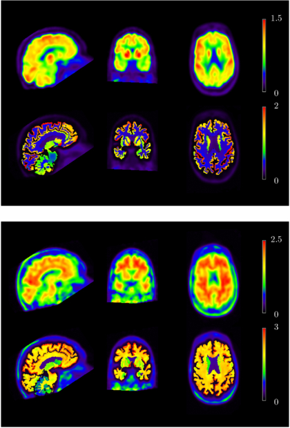
Figure 7. An 18F-FDG study (top panel) and a 18F-AV45 study (bottom panel) of the same AD subject before PVC (top row, each panel) and after RBV correction (bottom row, each panel). Images were normalized using cerebellar grey matter as reference region to generate standardized uptake value ratio (SUVR) images. Data provided by courtesy of Susan Landau and William Jagust (Jagust Lab, University of California, Berkeley).
Download figure:
Standard image
Figure 8. SUVR values for 18F-FDG (left) and 18F-AV45 (right) before PVC (uncorr.) and after RBV correction (RBV). Regional mean values for the precuneus, inferior temporal, superior frontal, posterior cingulate and sub-cortical white matter (WM) regions are shown.
Download figure:
Standard image3.4.2. Example 2: cardiology
As an example of the possible clinical value of PVC, an NCAT (Segars and Tsui 2002) body phantom was used in combination with a high-resolution contrast-enhanced gated cardiac CT image set to create both a cardiac perfusion SPECT study through Monte Carlo simulation (Ljungberg and Strand 1989) and co-registered templates for implementation of the modified template-reprojection method described in Pretorius and King (2009). The high-resolution contrast-enhanced gated cardiac CT was segmented as described by Pretorius et al (2002), using a greyscale histogram technique in combination with some thresholding. These image sets were averaged to form the basis of a non-gated cardiac perfusion study and the myocardium template respectively. The liver, lungs, and background (majority of other structures) from the NCAT phantom were inserted around the CT-based heart. Noise was added to the Monte Carlo simulated projections such that heart counts totalled 500 k for a 360° acquisition. Only 204 degrees worth of data were used in the reconstruction to simulate the IRIX gamma camera with Beacon transmission (Philips, Cleveland, OH) cardiac perfusion protocol. Emission data were reconstructed using the rescaled-block-iterative (RBI) method, a perturbation of ordered subsets expectation maximization (OSEM) with 17 subsets and 5/10 iterations with attenuation, triple energy window scatter and distance dependent resolution compensation included. The reprojected templates were similarly reconstructed without scatter compensation. Reconstructed sets of data were filtered using a three-dimensional Gaussian filter with a cutoff taking the voxel size into account (Pretorius and King 2009). PVC was performed, data reoriented to short axis slices, and polar map quantification performed using 17 myocardial segments according to the ASNC guidelines (Holly et al 2010). Results are given in figures 9, 10 and 11. The short axis slices in figures 9 and 10 show the importance of voxel size. PVC data in figure 9 (bottom row) are clearly a better representation of the true perfusion compared to the bottom row of figure 10. In figure 11, the uptake values together with the standard deviations are shown compared to the absolute truth. Only the template and data obtained using ten iterations are given. From the plots in figure 11 it is evident that even the heart template at the reconstruction voxel size, does not fully represent the true absolute perfusion value. The reason is twofold. First, the voxel size (3.12 mm) is still too coarse to describe the myocardium accurately at its thinnest parts, and second, the averaging due to cardiac gating adds additional blurring to the folded down heart template. It should be noted that the emission projections were acquired (simulated) using finer sampled source and attenuation maps (256 cube) of the NCAT phantom ensuring a more accurate description of the myocardium. Further study of all the data reveals that the average error compared to the template (best possible outcome) is an under estimation 11.1% ± 2.3% when five iterations are employed, improving to 9.6% ± 2.3% with ten iterations. Compared to the expected absolute perfusion value, these values deteriorate to 23.7% ± 6.8% and 22.4% ± 7.0% respectively. Results for the larger voxel size of 4.68 mm (not tabulated) are similar when compared to the template at that voxel size (12.7% ± 3.9% and 10.6% ± 3.9%), but worse compared to the expected absolute perfusion value (35.5% ± 7.6% and 33.8% ± 8.5%). Without PVC the average error for the two sets of voxel sizes ranges from 44.2% to 49.9%.
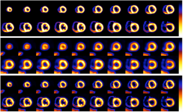
Figure 9. Short axis slices (3.12 mm voxels) of the heart template (top), RBI with attenuation, scatter, and resolution compensation after five iterations (middle), and PVC (bottom).
Download figure:
Standard image
Figure 10. Short axis slices (4.68 mm voxels) of the heart template (top), RBI with attenuation, scatter, and resolution compensation after five iterations (middle), and PVC (bottom).
Download figure:
Standard image
Figure 11. A graph depicting polar map quantification of the uptake values in the template, as well as in images reconstructed using RBI with ten iterations (with attenuation and resolution compensation) and RBI with ten iterations and PVC. Standard deviations are indicative of the uncertainty in the measurements. The truth (black line) represents the ideal case. Region 1 represents the apex, 2–5 represents the anterior, lateral, inferior, and septal apical regions respectively, 6–11 the anterior, antro-lateral, infro-lateral, inferior, infro-septal, and antro-septal mid-ventricular regions respectively, and 12–17 the basal regions.
Download figure:
Standard image3.4.3. Example 3: oncology
To illustrate the impact of PVC in PET tumour imaging, it is useful to examine how SUV varies when PVC is used. Images from patients with metastatic colon cancer are shown in figure 12. In the first patient, two rather large tumours can be seen in the selected slice (figure 12(A)). The tumour volumes estimated using an isocontour set to 40% of the maximum SUV in the tumours were 7.1 mL (tumour 1) and 10.3 mL (tumour 2). For the second patient (figure 12(B)), the tumour (tumour 3) was smaller (estimated volume of 1.4 mL). The images enhanced using a deconvolution approach (Lucy Richardson deconvolution assuming a 7 mm spatial resolution in the reconstructed images) are also shown in figure 12. For each tumour, four SUVs were calculated: SUVmax (SUV in the brightest voxel of the tumour), SUV40% (mean SUV in the tumour volume estimated using an isocontour set to 40% of SUVmax), SUV40% corrected for PVE using a RC (calculated based on the tumour volume estimated using the isocontour method), and SUVdecon defined as the mean SUV in the image enhanced by deconvolution (where the mean was calculated in a tumour volume estimated as an isocontour set to 70% of the maximum SUV in the original image (Teo et al 2007)). The corresponding values are shown in figure 13. These values illustrate the complexity of PVC in tumour imaging. The increase in tumour SUV due to PVC does not only depend on the tumour volume: although tumour 2 had a larger volume (10.3 mL) than tumour 1 (7.1 mL), the increase between SUV40% and SUV40%RC was greater for tumour 2 compared to tumour 1. This is because tumour 2 was less compact than tumour 1 due the presence of a large necrotic core. PVE was therefore more severe in tumour 2 than in tumour 1, as confirmed with the greater SUV increase in tumour 2 than in tumour 1 when comparing SUVdecon with SUVmax. The results also show that the SUV in the very small tumour 3 was greatly affected by PVC. In addition, figure 13 suggests that the PVC SUV still highly depends on which PVC method is used (substantial differences between SUV40%RC and SUVdecon). Still, the differences between PVC SUV tend to be smaller than the differences between uncorrected SUV (SUVmax and SUV40%). Obviously, the true SUVs for these tumours are unknown. Better understanding of the performance of the various PVC methods on real data and of the PVC impact on tumour assessment in the context of diagnosis and patient monitoring is strongly needed. PVC should now be offered as an option for tumour assessment, so as to facilitate investigations regarding the role of PVC in the context of tumour imaging.
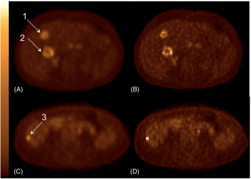
Figure 12. FDG PET slices of two patients with metastatic colorectal cancer. First patient (A) and (B) had two tumours while the second patient (C) and (D) had only one. Images were reconstructed with OSEM, 28 subsets and 2 iterations (A) and (C) and PVE was compensated for using image enhancement based on Lucy–Richardson deconvolution (B) and (D). Tumour's SUVs are presented in figure 13. Note the enhanced noise in the PV corrected images.
Download figure:
Standard image
Figure 13. SUV in the three tumours shown in figure 12, for different calculation methods with and without PVC (see text). The increase in SUV40% after RC-based PVC, as well as the increase in SUV between SUVmax and SUVdecon are given in parentheses above the corresponding bar. The tumour volumes are given in parentheses below the graph.
Download figure:
Standard image4. Discussion
There is growing interest in applying PVC and a growing awareness in the research community of its potential impact on image interpretation. To date vendors have been slow to implement turn-key PVC procedures, perhaps not surprising given that these often require effective inter-modality registration (often cross-vendor) and segmentation/parcellation as part of the correction procedure. The wider use of dual modality systems and introduction of PET/MRI should encourage the manufacturers to implement such methods on their consoles so that their clinical usefulness can be more broadly evaluated. Reliable correction can be challenging and needs care to ensure that the resolution of the reconstructed data (including any post-reconstruction processing) is consistent with the assumed resolution values in the correction procedure. This does introduce uncertainty that makes automation difficult. In this paper we have not addressed the problems of image registration and segmentation, but many useful algorithms have been reported in the literature; see e.g. Hutton and Braun (2003), Hutton et al (2006b), Slomka and Baum (2009), Klein et al (2009), Oliveira and Tavares (2012)) for registration and Boudraa and Zaidi (2006), Zaidi et al (2006), Zaidi and El Naqa (2010), Cabezas et al (2011) for segmentation algorithms.
In discussing PVC the underlying assumptions have been emphasised. For anatomically based methods, these include assumptions of perfect registration and segmentation as well as, in most cases, an assumption of uniform tracer distribution within parcellated sub-regions. Although recent developments attempt to address heterogeneity, these techniques require further development and validation. The sensitivity of PVC techniques to error in the underlying assumptions or pre-correction processing has not been fully documented for the complete range of available methods. Earlier papers did document the sensitivity to registration/segmentation errors of the MGM (Strul and Bendriem 1999) and GTM algorithms (Frouin et al 2002). Others have included some assessment of sensitivity to error but in general there is poor understanding as to which algorithms are most sensitive to these errors and hence which algorithms may be preferable in different situations. Obviously, deconvolution-type methods that do not rely on anatomical data are insensitive to these errors.
To accurately measure uptake in small structures is challenging, although tracer concentration can theoretically be estimated for small structures, provided there is a clear understanding of the underlying structure where the tracer is distributed in relation to surrounding sources of activity; for example PVC is applied to estimation of uptake in plaque in large vessels or in atrophied grey matter. Careful attention to variations in PSF requires knowledge of the effects on resolution of depth of interaction, positron transport in non-homogeneous materials, septal penetration effects at different energies as well as possibly detector-specific properties (e.g. in solid state detectors). In most cases these finer details are ignored, assuming they have only secondary influence; PVC that takes account of these factors remains complex. Correction for motion also becomes more critical for small structures but, as stated earlier, is beyond the scope of this review.
Although not specifically addressed in this review, PVC is even more challenging in preclinical imaging (e.g. rodents) where structures are extremely small relative to the achievable resolution on preclinical scanners (∼0.35 mm for SPECT or ∼0.9 mm for PET). There is little published on PVC on these systems. For PVC in small animal imaging it may be important to take into account the spatial variation of the PSF as well as the positron range in the case of PET. Clearly any variation in resolution across the field-of-view becomes quite critical (Lehnert et al 2011a, Szanda et al 2011), as does positron range effects (Lehnert et al 2011b). Incorporation of positron range effects as a component of partial volume correction algorithms has received limited attention to date, although several groups have worked on incorporating positron range within iterative reconstruction (e.g. Fu and Qi 2008, Alessio and MacDonald 2008).
In this work we have focused on PVC methods based on a model of the spatial distribution of image values, as described by the PSF of the system. However, we should also mention that PVC methods have also been developed based on statistical models for the distribution of image values in an intensity histogram (Santago and Gage 1995, Wells et al 2007). This approach does not require anatomical information.
There have been few studies that cross-compare the effectiveness of the various methods or evaluate robustness; clearly an area where there is room for further investigation. As with other correction techniques (e.g. scatter correction) the end user can be confused by the range of available methods and unclear as to which approach is recommended. There is understandably concern in the clinical community regarding the interpretation of PV corrected studies; for example, as emphasized in the oncology section, the removal of volume effects can reduce the observable changes in SUV in response to treatment. Similarly PV corrected, gated cardiac studies would no longer illustrate 'brightening' during contraction as a result of myocardial wall thickening. However, the observed intensity after PVC reflects unambiguously the tracer uptake independent of underlying volume/thickness and will therefore be more sensitive to true changes in tracer uptake rather than influencing factors, such as volume or tissue components that contribute to the tissue fraction. PVC is an important correction to ensure that measurements are truly quantitative.
Having said this, we should also point out that image noise and noise correlations, as well as the precision of quantitative estimates of activity, are measures that can often be equally important as image fidelity or quantitative accuracy, and therefore it is crucial that investigators working on existing or new approaches to PVC also evaluate and report on the noise handling of the methods, in addition to their accuracy. Also the sensitivity of PVC techniques to error in pre-correction processing steps, such as registration and segmentation should be evaluated. Some of the issues are addressed in a recent study comparing a number of different PVC and anatomically guided reconstruction methods (Hutton et al 2012).
5. Summary
A large number of different methods for PVC have been proposed in the past. Some methods utilize anatomical information, some do not. Some methods produce only mean values for one or more regions, some perform a voxel-by-voxel correction for a region or the whole image. Some methods are applied to a reconstructed image; some are incorporated in the reconstruction algorithm. Although these PVC methods were originally developed for cardiology, neurology or oncology with either PET or SPECT, most methods are applicable in multiple areas. PVC is an important aspect of quantitative analysis in emission tomography, which remains an area of active research. The clinical community should be encouraged to adopt PVC methods as part of standard processing procedures. Multimodality systems, combining PET or SPECT with CT or MRI, allow acquisition of co-registered functional and anatomical images. As these systems are becoming widely available, perhaps the time has come for PVC to be routinely used in clinical practice.
Acknowledgments
We want to thank Susan Landau and William Jagust (Jagust Lab, University of California, Berkeley) for kindly providing data for one of the clinical examples. IB thanks JA Maisonobe for helping with the preparation of some figures. We would also like to thank an anonymous reviewer, whose constructive criticism helped improve this paper. KE is supported by a centre grant jointly funded by Cancer Research UK (CRUK) and EPSRC. BH is partly supported by a grant from the Engineering and Physical Sciences Research Council, EP/G026483/1. UCLH/UCL receives a proportion of its funding from the UK Department of Health's NIHR Biomedical Research Centre's funding scheme.